Sparse Networks and Lottery Winners
Sparse Networks and Lottery Winners
It’s really easy to train an artificial neural network to classify articles of clothing, as long as you’re not too picky.
If you want to get technical, a two-layer perceptron with just 12 hidden neurons can easily be trained on the Fashion-MNIST dataset to an accuracy of above 80%. Ten passes through the dataset is more than enough to max out the model’s capacity to learn.
Epoch  1/10, Accuracy: 75.35%
Epoch  2/10, Accuracy: 80.50%
Epoch  3/10, Accuracy: 81.46%
Epoch  4/10, Accuracy: 81.93%
Epoch  5/10, Accuracy: 82.29%
Epoch  6/10, Accuracy: 82.87%
Epoch  7/10, Accuracy: 83.35%
Epoch  8/10, Accuracy: 83.38%
Epoch  9/10, Accuracy: 82.90%
Epoch 10/10, Accuracy: 83.35%
Our model’s not a genius, but it can reliably separate shirts from shoes four times out of five and I think that’s pretty good for just a few minutes.
But now that we’ve trained this model, I’m curious about what’s going on inside it. In particular, I’m curious about the model’s weights.
Weighty Matters
Weights describe how strongly connected each neuron is to the neurons in the next layer. A weight with a big value means whatever comes through it gets amplified; a small value means it gets dialed down. So really it’s the weights that define the topology of the neural network. They’re what determines what connects to what.
Normally when you train a model, you start by initializing it in a particular way that makes the numbers mostly evenly distributed and mostly quite small. So at the start, every neuron is a little bit connected to every neuron in the next layer.
Training changes these weights. Some go up, get stronger — represent a stronger connection between layers. Some go down, get weaker.
So let’s do some basic statisics on these weights and see what we can learn.
Analyzing trained weights...

=== Weight Statistics ===
Total weights: 6344
Mean: -0.004816
Std Dev: 0.158104
Min: -1.124022
Max: 0.924387

=== Percentage of weights by absolute value ===
|w| < 0.001: 0.66%
|w| < 0.01: 5.88%
|w| < 0.05: 29.11%
|w| < 0.1: 53.92%

Generating trained weight plots...
Saved weight histogram to ./plots/trained_weight_histogram.png
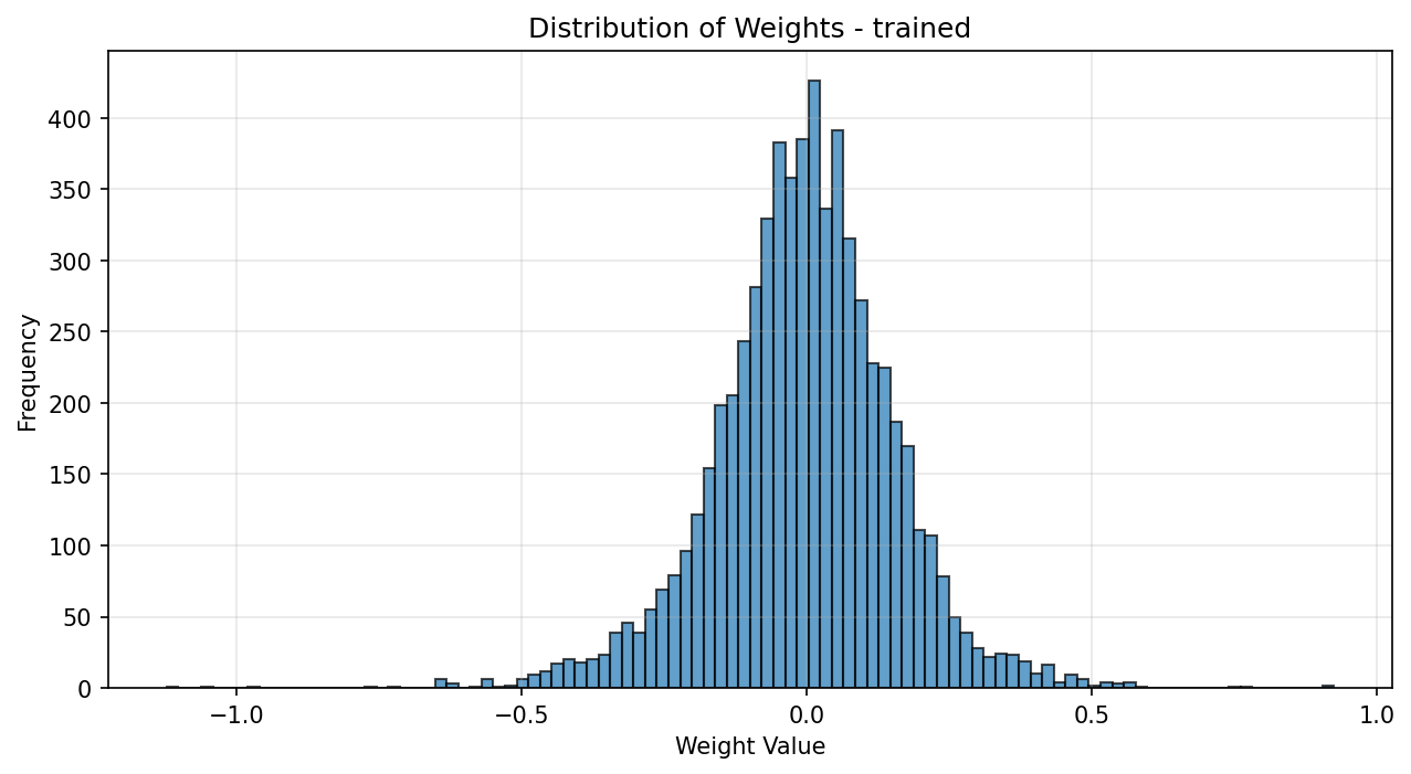
Now I am not a statistician; this right here is the absolute outer limit of my statistics expertise. I get what standard deviation does qualitatively, and I know how to read a histogram — more or less. But you know what immediately jumps out to me about these weights?
There’s a whole lotta nothin’ here.
By which I mean look, half the weights have a magnitude of less than 0.1, and almost a third are smaller than 0.05. That’s thousands of neurons that aren’t passing much on to the next layer downstream.
What difference would it make — a lot or a little — if instead of close to zero they were exactly zero?
Let’s find out.
What we’ll do is split the weights up into percentile bands ten points wide, then we’ll start zeroing them out from the least signifiant 10% all the way up.
Pruned   0th percentile | |w| < 0.0000 | Sparsity:   0.0% | Params: 6344/6344 | Accuracy: 83.35%
Pruned  10th percentile | |w| < 0.0163 | Sparsity:  10.0% | Params: 5709/6344 | Accuracy: 83.35%
Pruned  20th percentile | |w| < 0.0339 | Sparsity:  20.0% | Params: 5075/6344 | Accuracy: 83.22%
Pruned  30th percentile | |w| < 0.0511 | Sparsity:  30.0% | Params: 4441/6344 | Accuracy: 82.63%
Pruned  40th percentile | |w| < 0.0703 | Sparsity:  40.0% | Params: 3806/6344 | Accuracy: 78.94%
Pruned  50th percentile | |w| < 0.0899 | Sparsity:  50.0% | Params: 3172/6344 | Accuracy: 75.67%
Pruned  60th percentile | |w| < 0.1166 | Sparsity:  60.0% | Params: 2538/6344 | Accuracy: 76.20%
Pruned  70th percentile | |w| < 0.1469 | Sparsity:  70.0% | Params: 1903/6344 | Accuracy: 67.34%
Pruned  80th percentile | |w| < 0.1839 | Sparsity:  80.0% | Params: 1269/6344 | Accuracy: 60.51%
Pruned  90th percentile | |w| < 0.2494 | Sparsity:  90.0% | Params:  635/6344 | Accuracy: 32.75%
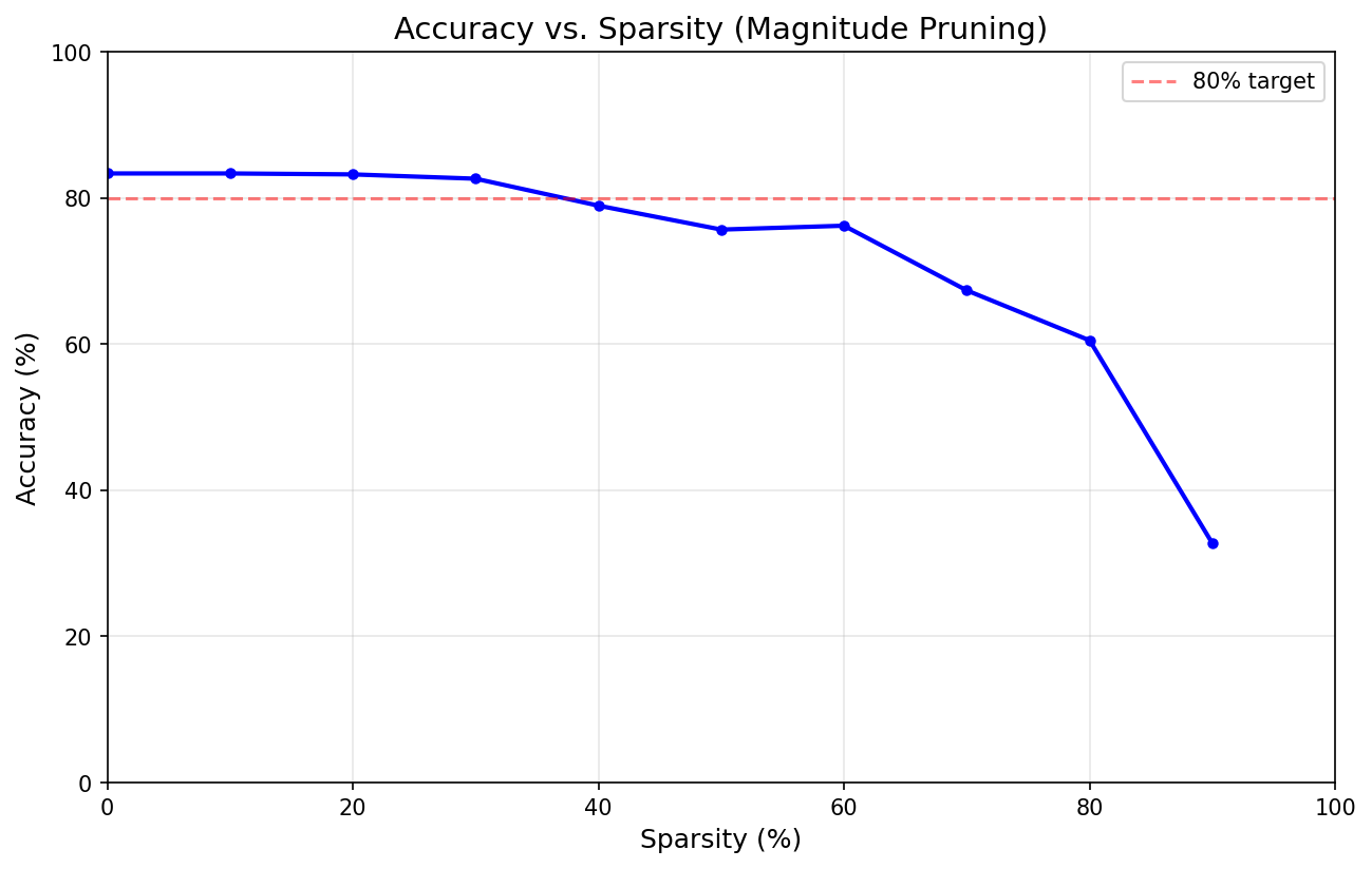
Do you see how the model accuracy stayed high through losing the bottom thirty percent of its weights? There’s not even a significant dip until a sparsity of 40 percent — that’s four out of every ten connections cut.
It seems like about thirty percent of the weights in our model kind of aren’t doing anything. I mean, they’re doing something, but their contributions are so insignificant that they might as well be zero.
This is not a new idea. That neural networks can be pruned to go from dense (all weights non-zero, every neuron connected to every one in the next layer) to sparse (some weights zero, some connections severed) dates back at least as far as 2017 when it was written about by Li et al. in “Pruning Filters For Efficient ConvNets.” Their specific work was on convolutional neural networks, but the idea applies equally well — as I think I’ve just demonstrated — for simple multilayer perceptrons as well.
Just how far can these networks be pruned, though? We got down to a sparsity of 30% with no measurable decline in quality. Can we do better?
Turns out yeah.
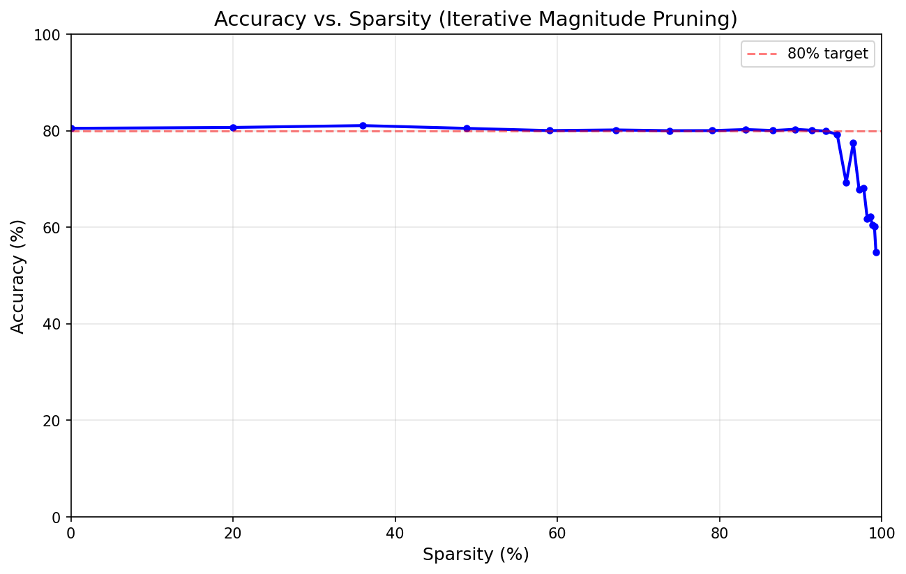
Here we see a plot of accuracy as a function of sparsity, just like the figure above. But look how different the plot is. Instead of a little lip and then from about 30 percent a smooth downward-trending arc, this time the accuracy stays practically flat to a sparsity of almost 95 percent.
We severed roughly 19 out of every 20 layer-to-layer connections in that model and it still worked. That’s like breaking 84 of the 88 keys on a piano and still being able to play a tune.
Lemme try to explain how.
The Lottery Ticket Hypothesis
In 2019 Frankle and Carbin from MIT advanced the Lottery Ticket Hypothesis: “A randomly-initialized, dense neural network contains a subnetwork that is initialized such that — when trained in isolation — it can match the test accuracy of the original network after training for at most the same number of iterations.”
What that means is basically what we’ve said so far: Inside every trained neural network there’s a subnetwork that’s special, that does the actual work. If you can identify that subnetwork, you can go back to the beginning and train just that subnetwork to be as good at your task as the whole network could have been with no more extra training.
If you can identify that subnetwork.
Well, Frankle and Carbin had an idea about that too. It took the form of a simple algorithm:
- Initialize a dense model to some randomized state which we’ll call θ₀.
- Train that model to your desired degree of doneness.
- Identify and mask out the least significant weights.
- Reset the now-sparse model to its original θ₀ state.
- Train the model again.
- Repeat until you can no longer meet your training criterion.
That’s what I did to produce the plot shown above. I took the original 6,344-weight model and set it to state θ₀, then trained it up — this is the exact same thing I did to kick this all off, if you’ll recall. But then I identified the bottom 20% of weights by magnitude and masked them out, reset to θ₀, then retrained. Repeat until the pruned model can’t be trained up to at least 80% accuracy.
The result was a 544 weight, 91.4% sparse model that trained up in nine iterations to an accuracy of 80.09%.
Does that mean that any 544-weight, 91.4% sparse model with this architecture can be trained up in nine iterations to 80.09% accuracy? No. With a different θ the same sparse network fails to hit the accuracy goal even after four times as many training iterations.
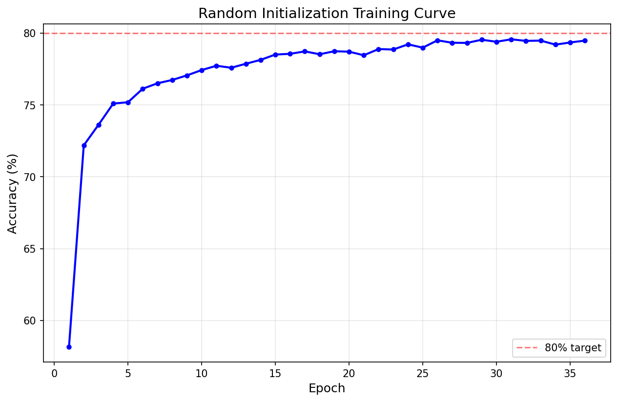
So it’s not just the topology of the network. It’s also the initial state of the network. Given this initial state θ₀, there exists within the dense network a sparse subnetwork that’s capable of being trained to do your task. That’s just the Lottery Ticket Hypothesis in different words.
But … why? When we first initialized our model back at the very beginning, we baked into it the solution to our problem. How did we do that? How did we get lucky enough to do that? And why don’t you ever hear about neural network training … failing? What happens if the initialized network doesn’t contain the solution to your problem?
The answer has to do with big numbers.
It’s Basically Predestination But For Matrices
Imagine you’re at the roulette table. You’ve bet it all on lucky 13. The wheel’s spinning, and the croupier is about to drop the ball. What are your odds? By the book, in a fair game, they’re 1 in 37.
But what if you dropped two balls? Then your odds would go up to two in 37, or about 5 percent.
If you dropped 25 balls you’d have almost a 50/50 chance of winning. Did you know that? Fun fact.
So what if you played a hundred times? Your odds of not having won by that time would be just about six percent.
And if you played a thousand times? Your odds of not winning in all that time would be about one in a trillion.
How does all this relate to machine learning? Machine learning uses large numbers to cheat at the game.
See, when you create a dense network, you’re simultaneously creating all the sparse network that that dense network contains. And dense networks are roomy. Let’s do some quick back of the envelope calculations: Our original neural network — 784 inputs, 8 neurons, 4 neurons, 10 outputs — had:
- Layers 1-2: 784 × 8 = 6,272 weights
- Layers 2-3: 8 × 4 = 32 weights
- Layers 3-4: 4 × 10 = 40 weights
- Total: 6,344 weights
Once we pruned it down, our “lottery winner” sparse network had 544 weights.
So what we essentially did was create a bunch of 544-weight sparse subnetworks inside one big 6,344-weight dense network, and then during the training process we searched them all in parallel, essentially, to find the one that would solve our problem.
Neat!
But that doesn’t answer our question about why training never seems to fail. I mean sure, there are plenty of ways to fail to train a network, but as long as you have trainable data and good architecture for your problem, training is guaranteed to find you a solution first time out. How does that work?
Well it’s not really true to say that training is guaranteed to find a solution. But it turns out that it is true that the odds of failing to find a solution … well, remember the roulette wheel? It’s like betting it all on lucky 13 a thousand times in parallel. You’d have to beat one-in-a-trillion odds not to win in that case.
That’s how training works. It’s like betting it all on lucky 13 a bunch of times in parallel, thereby increasing your odds of finding a winner.
How many times?
Well like I said, we created a 6,344-weight dense network, and then we searched all the 544-weight sparse networks inside that dense network in parallel. So the question is, how many 544-weight networks are there inside a big 6,344-weight network?
I’ll just skip to the end because the math has factorials in it. It’s 10 to the 1,089 power.
That’s how many times we dropped the ball. That’s how many lottery tickets we bought. Ten to the thousandth power.
That’s how big that number is, by the way. I just dropped 89 orders of magnitude off the end and I don’t care. You can just do things.
There are about 10 to the 100 atoms in the observable universe. For every atom, there’s about 10 to the 900 544-weight sparse subnetworks inside the 6,344-weight dense network.
See? The numbers are just pointless. That was what we got from basically 1,000 choose 100. Modern large language models are more on the order of a trillion choose a billion. Just hilariously off-the-scale big numbers.
In Which He Gets To The Point
This is why artificial neural networks work.
Even if your problem is very hard, even if the odds of finding a solution are very small, if you throw 10 to the 1000 solutions at it, you’re almost sure to get a working one, and probably pretty quickly in the cosmic scheme of things.
This is the fundamental trick that makes artificial neural networks possible. This is how we cheat at the game. Combinatorics and graph theory and subnetworks and big, big, just stupidly big numbers.
https://github.com/Embedding-Space/sparse-networks-and-lottery-winners